Here, we specify the county (or groups of counties), state, year, and affordability cutoffs to analyze. This allows us to easily create reports for different times, places, and scenarios.
Our analysis relies on the 2022 PUMS dataset from the US Census. We fetch the data directly from the Census API, and only grab a handful of the variables available within PUMS (vars).
In [5]:
vars <-c("BLD", "PUMA", "HFL", "TEN", "YRBLT", "HINCP", "NP", "MV", "BDSP", "ELEP", "FULP", "GASP", "MRGP", "RNTP", "RMSP", "ELEFP", "FULFP", "GASFP")# Get data from the Census APIpums_path <-paste0("/mnt/data/pums_1_22_", STATE_FIPS, ".Rds")# Get data from the Census APIif (file.exists(pums_path)) { raw_data <-readRDS(pums_path)} else { raw_data <-get_pums(variables = vars,state = STATE_FIPS,year =2022,survey ="acs1",rep_weights ="housing",recode =TRUE) |>distinct(SERIALNO, .keep_all =TRUE) # housing units only, not peoplesaveRDS(raw_data, pums_path)}
Owned with mortgage or loan (include home equity loans)
03102
73800
2
Valid monthly electricity cost in ELEP
230
No charge or gas not used
3
No charge or fuel other than gas or electricity not used
2
5
20-49 Apartments
2
1970 to 1979
Rented
04003
170000
1
Valid monthly electricity cost in ELEP
400
Valid monthly gas cost in GASP
40
No charge or fuel other than gas or electricity not used
2
18
One-family house detached
4
1960 to 1969
Owned with mortgage or loan (include home equity loans)
00703
190000
4
Valid monthly electricity cost in ELEP
300
Valid monthly gas cost in GASP
300
No charge or fuel other than gas or electricity not used
2
26
One-family house detached
4
1990 to 1999
Owned with mortgage or loan (include home equity loans)
00901
77000
1
Valid monthly electricity cost in ELEP
130
Valid monthly gas cost in GASP
330
No charge or fuel other than gas or electricity not used
2
24
10-19 Apartments
2
1990 to 1999
Rented
03308
16800
1
Valid monthly electricity cost in ELEP
60
Valid monthly gas cost in GASP
80
No charge or fuel other than gas or electricity not used
2
22
N/A (GQ)
-1
NA
N/A (GQ/vacant)
00905
-60000
1
N/A (GQ/vacant)
2
N/A (GQ/vacant)
3
N/A (GQ/vacant)
2
0
One-family house attached
3
1939 or earlier
Owned with mortgage or loan (include home equity loans)
04111
34300
2
Valid monthly electricity cost in ELEP
100
Valid monthly gas cost in GASP
110
No charge or fuel other than gas or electricity not used
2
15
N/A (GQ)
-1
NA
N/A (GQ/vacant)
02500
-60000
1
N/A (GQ/vacant)
2
N/A (GQ/vacant)
3
N/A (GQ/vacant)
2
0
One-family house attached
3
1990 to 1999
Owned with mortgage or loan (include home equity loans)
03902
313000
4
Valid monthly electricity cost in ELEP
220
Valid monthly gas cost in GASP
150
No charge or fuel other than gas or electricity not used
2
16
One-family house detached
3
1939 or earlier
Owned free and clear
03313
40600
2
Valid monthly electricity cost in ELEP
70
Valid monthly gas cost in GASP
50
No charge or fuel other than gas or electricity not used
2
44
PUMS consists of so-called “microdata”: anonymized, individual-level households survey results. Every row contains the answers that a real person gave on a questionnaire. For our purposes, the key variables are:
variables
example value
description
HINCP
$113,000
The household’s income over the past 12 months
ELEP
$170
The household’s monthly electricity cost
GASP
$80
The household’s monthly natural gas cost
FULP
$100
The household’s annual cost for fuels other than electricity and natural gas
For definitions of other PUMS variables, consult the official data dictionary. To learn how to work with PUMS data, check out this tutorial.
PUMAs
What if we want to calculate the average annual income of a specific area? PUMS doesn’t tell us the city or county each household is located in, only the public use microdata area (PUMA).
PUMAs are Census geographies that contain at least 100,000 people and are entirely within a single state. They are built from census tracts and counties, and may or may not be similar to other recognized geographic boundaries. (So, if you are interested in pulling data about block groups, census tracts, or other small areas, you can’t use PUMS data.)
In densely populated areas like New York City, PUMAs are closely aligned to Community Districts, which are smaller than counties. In some places, PUMAS are equivalent to counties. In the least populated places, a single PUMA can span several entire counties. These scales are granular enough for our purposes.
PUMAS to counties
PUMAs are represented by numeric codes like 01101 (see the PUMA column above). Reporting the number of energy burdened families for PUMA 01101 won’t mean anything to anyone, so need to associate PUMAS with counties in order make our results digestible to readers. Let’s import a PUMA-to-county mapping.
Rows: 187 Columns: 9
── Column specification ────────────────────────────────────────────────────────
Delimiter: ","
chr (4): PUMA (2012), State abbr., County name, PUMA12 name
dbl (5): State code, County code, Total housing units (2020 Census), county-...

ℹ Use `spec()` to retrieve the full column specification for this data.
ℹ Specify the column types or set `show_col_types = FALSE` to quiet this message.
puma_county_mapping |>head() |>gt()
state_code
puma_2012
county_code
state_abbr
county_name
puma12_name
total_housing_units_2020_census
county_to_puma12_allocation_factor
puma12_to_county_allocation_factor
36
00100
36089
NY
St. Lawrence
St. Lawrence County
51612
1
1.0000
36
00200
36019
NY
Clinton
Clinton, Franklin, Essex & Hamilton Counties
37315
1
0.3904
36
00200
36031
NY
Essex
Clinton, Franklin, Essex & Hamilton Counties
25123
1
0.2628
36
00200
36033
NY
Franklin
Clinton, Franklin, Essex & Hamilton Counties
25318
1
0.2649
36
00200
36041
NY
Hamilton
Clinton, Franklin, Essex & Hamilton Counties
7826
1
0.0819
36
00300
36113
NY
Warren
Warren & Washington Counties
39928
1
0.5793
One PUMA may be associated with several low-population counties: in the example above, PUMA 00200 is associated with Clinton, Essex, and Franklin counties. (The reverse situation can also occur: Queens county is made up of several geographically small PUMAS, each with a population of roughly 100,000 people.)
If our goal is to calculate the energy burdens for each county, this presents a problem: we can calculate metrics for a PUMA, both how do we break them down for each constituent county? We’ll use each county’s puma12_to_county_allocation_factor, which simply reflects the percentage of the PUMA’s population found in that county.
LMI cutoffs
Finally, we want to report our findings in terms the Area Median Income (AMI). AMI is defined as the midpoint of a particular area’s income distribution, which is calculated every year by the Department of Housing and Urban Development (HUD).
The “Area” in Area Median Income is the county. 80% is the cutoff associated with Low and Moderate Income (LMI) households. Let’s import a dataset from HUD that lists 80% of each county’s AMI.
Note that AMI isn’t defined as the median income of all households in a given county. There’s actually an AMI for each household size (the NP column for number of persons).
In the example above, the LMI cutoff in Albany county for a two-person household is $61,200, for a three-person household is $68,850, and so on. This represents the median household income of all 2-person households in the county, multiplified by .8.
Calculate household-level burdens and savings
With our datasets imported, we can construct the household-level variables we need for our analysis.
In [9]:
data <- raw_data |>filter(HINCP >0) |># Remove surveys that didn't report income (0). We assume non-respondense is uncorrelated with income.# Negative income usually means a business loss, and that is both rare and not relevant for our purposesmutate(# Denote if responded reported any energy costs or notbill_in_rent = (ELEFP =="1") | (GASFP =="1") | (FULP =="1"),# ACS uses low values of these columns to denote different reasons for zeros, not actual values, so we need to set them to zeroGASP =case_when(GASP <=4~0, .default = GASP),ELEP =case_when(ELEP <=3~0, .default = ELEP),FULP =case_when(FULP <=3~0, .default = FULP),# Calculate household's yearly energy billyearly_energy_bill = (ELEP + GASP) *12+ FULP,# Find household's energy burden percentage, whether they're burdenedenergy_burden_pct = yearly_energy_bill / HINCP,is_energy_burdened = energy_burden_pct > burdened_cutoff,# Find difference between how much household must spend on energy# to be burdened, and how much they actually spendburdened_income_cutoff = burdened_cutoff * HINCP,annual_energy_burden = yearly_energy_bill - burdened_income_cutoff,monthly_energy_burden = annual_energy_burden /12,# NY HEAT only applies to electricity and gas, not delivered fuels.# Repeat burden calculation for utility energy alone.yearly_utility_bill = (ELEP + GASP) *12, # `utility` bill does not include delivered fuelutility_burden_pct = yearly_utility_bill / (HINCP+1),monthly_utility_burden = (yearly_utility_bill - (burdened_cutoff * HINCP)) /12,is_utility_burdened = utility_burden_pct > burdened_cutoff) |>filter(!bill_in_rent)
Next, we link households to counties through PUMAs. This will cause households that live in PUMAs that span multiple counties to be duplicated, which we deal with later on. We also bring in each county’s LMI cutoff and economic region.
The survey responses in PUMS come from a sample of the population in each PUMA. To report statistics about the PUMA as a whole, and therefore for counties, we need to us special weights supplied by the Census (the WGTP column).
And because one PUMA may map to multiple columns, the weight for each PUMS record actually comes from combining two separate weights: WGTP from the ACS, which tells us how much to weight a given observation for a given PUMA, and puma12_to_county_allocation_factor that tells us how to allocate a PUMA to a county.
For instance, for a PUMA that is totally contained within a county, this value will just be WGTP, but if a PUMA is split 50% between two counties, then each observation would be WGTP times 0.5.
In [10]:
data <- data |>inner_join(puma_county_mapping, by =c("PUMA"="puma_2012"),relationship ='many-to-many') |>mutate(wt = WGTP * puma12_to_county_allocation_factor) |>inner_join(county_lmi, by =c("county_name"="County", "NP")) |>mutate(is_lmi = HINCP <= lmi_cutoff) |>filter(county_name %in% county_names, wt >0)
For flexibility, each row can either be generically called “Area”, or else it can get a region name.
In [11]:
# Depending on whether we've got multiple groups or not, we add another labelif (length(region_groups) >1) { data <- data |>right_join(region_mapping, by ="county_name")} else { data$region_group <-"Area"}
We know whether each household in our sample is_energy_burdened: whether they pay more than 6% of their annual income on energy.
We’ve also calculated their energy_burden_pct: the percent of their income they actually spend on energy.
We also know their utility_burden_pct and is_utility_burdened: what percent of their annual income they’re spending on electricity and natural gas bills alone–excluding delivered fuels–and whether this exceeds 6% of their annual income.
Finally, we’ve calculated how much money utility-burdened households would save every month (monthly_utility_burden) if their bills were downsized to just 6% of their income.
Aggregate burdens and savings across the state
All that’s left now is to report the following metrics for different geographies, starting with the entire state:
households_included: the number of households
median_income: the median income of households in the geography
pct_energy_burdened: the percent of households that are energy burdened
avg_monthly_bill_of_burdened: the average monthly energy bills of those households, before NY HEAT
utility_burden_of_burdened: how much utility burdened households stand to save every month, after NY HEAT
In [13]:
total_rollup <- data |>summarise(households_included =sum(wt),median_income = Hmisc::wtd.quantile(HINCP, weights = wt, probs =0.5),pct_energy_burdened =weighted.mean(is_energy_burdened, w = wt),pct_utility_burdened =weighted.mean(is_utility_burdened, w = wt),avg_monthly_bill_of_burdened =weighted.mean(case_when( is_energy_burdened ~ yearly_energy_bill /12), w = wt,na.rm =TRUE),utility_burden_of_burdened =mean(case_when( is_utility_burdened ~ monthly_utility_burden), w = wt,na.rm =TRUE)) |>mutate(region = REGION_NAME,grouping ="Total")
Next, we crunch the same numbers for each PUMA:
In [14]:
puma_rollup <- data |>summarise(households_included =sum(wt),median_income = Hmisc::wtd.quantile(HINCP, weights = wt, probs =0.5),pct_energy_burdened =weighted.mean(is_energy_burdened, w = wt),pct_utility_burdened =weighted.mean(is_utility_burdened, w =wt),avg_monthly_bill_of_burdened =weighted.mean(case_when( is_energy_burdened ~ yearly_energy_bill/12), w = wt,na.rm =TRUE),utility_burden_of_burdened =mean(case_when( is_utility_burdened ~ monthly_utility_burden), w = wt,na.rm =TRUE),.by =c(puma12_name, PUMA)) |>filter(households_included >=5000) |>mutate(grouping ="Area",unit_id =paste0(STATE_FIPS, PUMA)) |>rename(region = puma12_name)
In [15]:
county_rollup <- data |>summarise(households_included =sum(wt),median_income = Hmisc::wtd.quantile(HINCP, weights = wt, probs =0.5),pct_energy_burdened =weighted.mean(is_energy_burdened, w = wt),pct_utility_burdened =weighted.mean(is_utility_burdened, w =wt),avg_monthly_bill_of_burdened =weighted.mean(case_when( is_energy_burdened ~ yearly_energy_bill/12), w = wt,na.rm =TRUE),utility_burden_of_burdened =mean(case_when( is_utility_burdened ~ monthly_utility_burden), w = wt,na.rm =TRUE),.by =c(county_name, region_group)) |>filter(households_included >=5000) |>mutate(grouping = region_group,unit_id = county_name) |>rename(region = county_name)
Tabulate burdens and savings across the region
Let’s place each level of rolled-up metrics into a single table we can embed into the report.
In [16]:
rollup <-function(component_rollup) {bind_rows(total_rollup, component_rollup) |>mutate(region =str_replace(region, "^.*Community", "Community")) |>select(region, grouping, pct_energy_burdened, avg_monthly_bill_of_burdened, utility_burden_of_burdened) |>group_by(grouping) |>gt() |>row_group_order(c("Total", region_groups)) |>fmt_currency(c(avg_monthly_bill_of_burdened, utility_burden_of_burdened), decimals =0) |>fmt_percent(c(pct_energy_burdened), decimals =0) |>cols_label(region ="Region",pct_energy_burdened ="Homes with high energy burdens (%)",avg_monthly_bill_of_burdened ="Avg. monthly energy bills of high-burden homes",utility_burden_of_burdened ="Avg. monthly savings for high-burden homes under NY HEAT", ) |>tab_footnote("Excluding households with utility bills in rent, or missing fuel or income information.\nSource: 2022 ACS. Win Climate, 2024")}
In [17]:
if (REPORT_TYPE =="county") { tbl_results <-rollup(puma_rollup)} else { tbl_results <-rollup(county_rollup)}tbl_results
Region
Homes with high energy burdens (%)
Avg. monthly energy bills of high-burden homes
Avg. monthly savings for high-burden homes under NY HEAT
Total
Albany County
19%
$259
$114
Area
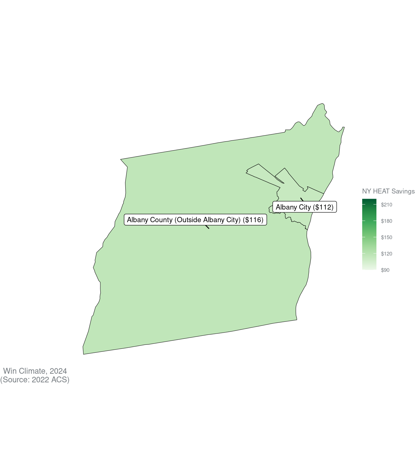
Albany County (Outside Albany City)
16%
$274
$116
Albany County (East Central)--Albany City
24%
$238
$112
Excluding households with utility bills in rent, or missing fuel or income information. Source: 2022 ACS. Win Climate, 2024
Map burdens and savings across the region
Now, let’s create some maps of our metrics.
Let’s create some map-creation functions that we can reuse.